FlexMeasures Releases v0.18, with Better Use of Future Knowledge

Version 0.18 of FlexMeasures advances the modeling of the flex optimization problem, adding more detail. If we have knowledge about future conditions and underlying physics, our optimization gets better when we put that to use!

We also improved navigation in the UI, which is really handy for more complex asset structures.

See the changelog for a complete list. Read on below about the larger new features we added.

FUTURE KNOWLEDGE IN SCHEDULING

FlexMeasures lets you describe the underlying flexibility problem, so that the internal scheduler knows within what limits to work to find the best solution for the upcoming hours. Earlier, we introduced two data specifications for this, the flex-model (what are the limits and goal around this asset, e.g. maximal state of charge?) and the flex-context (what is also relevant, e.g. prices?). We wrote a tutorial with nice examples around the V2G use case.

Now. we have enhanced the flex-model with three new (or more nuanced) types of information, which lets FlexMeasures handle a wider range of modern energy flexibility problems. We also let them be sensors, instead of just one constant value. But more about that later, first let me introduce the new kinds of flex-model information:

EXTERNAL IN- AND OUTPUT FOR STORAGE

We can model storage assets which only serve the flexibility of the main system, e.g. a battery which only exists to simply buffer solar energy for self-consumption at some later time. The battery has no strict dependencies outside of our energy flexibility asset model.

But often, storage (also) serves an external and crucial purpose. A good example is a hot water tank. Comfort of the home occupants is the main goal, consuming energy to create heat at the best time is also important, but secondary.

Thus, the expected extraction of energy (as heat) from the storage is an important input to the modeling problem ― it will form a constraint. In this example, the input of energy (as electricity) is dynamic, and can be timed optimally to lower the energy costs and/pr CO2.

To handle these situations optimally, we introduced fields in the flex model to represent an expected extraction of stored energy (e.g. when we know the occupants are at home), or even addition (e.g. when an industrial process will add heat) ― we called them soc-usage and soc-gain. This makes the flex model much more expressive. Obviously, these fields only work with the StorageScheduler.

ENERGY CONVERSION EFFICIENCY

CONSUMPTION AND PRODUCTION CAPACITIES

Until now, only one kind of maximal capacity was possible (for example, to describe a limit to the grid connection). We used the field power-capacity, and it had to have one constant value, e.g. 25 kW.

{
    "flex-model": {
        "consumption-capacity": "25 kW",
        "production-capacity": {"sensor": 51}
    }
}

We can now differentiate between limits on production and consumption. power-capacitystill works ― if it is given, it would serve as a limit on the other two.

This work was done in Pull Requests 906, 933 and 897.

UI NAVIGATION OF COMPLEX SITES

Behind the scenes, we work with more complex asset structures. We have introduced the capability of assets being the child of another asset. Now, tree-like structures can be built (where sensors are the leaves, usually) in order to model whole sites or different scenarios for simulation projects.

This also calls for efforts to navigate this structures. We are looking to develop a visual representation of this tree-structure. But until we get there, we made it easier to navigate the structure.

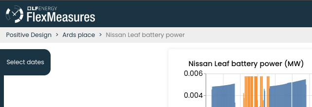
First, we introduced a breadcrump-bar above the asset and sensor pages. This example has the account, the asset and the currently shown sensor:

Second, we made lists of assets and sensors easy to click. The whole row will now react to one simple click and take you where you want to go!

This work was done in Pull Request 930 and 923.